This web has migrated to github on the following link
Upgrade Debian Wheezy to Debian Jessie
In this last week, I updated my RStudio in Debian Wheezy and it turned out that it needed a more recent version of the package lib6. A reliable solution was to upgrade my system to Jessie, the current stable distribution of Debian. Its latest update, Debian 8.1, was released on 6th of June, 2015.
For this reason, I share, in this post, the steps I followed for upgrading my system keeping user configuration and the main programs I use such as R, RStudio, Matlab, Mendeley, TeXstudio and others.
0) Backup your data: This is a logical initial step before starting any change on the system.
1) Upgrading to Debian Jessie:
1.1) Prepare Debian Wheezy to be upgrading: Be sure that your current system does not have any problem of dependency or wrong installed packages. You can use the following commands for that purpose:
# Login like super user and write your password
su -
# Prepare your system
aptitude update
aptitude upgrade
aptitude dist-upgrade
1.2) Update the repositories list: Packages for Debian Jessie is downloaded from these repositories. One way to update this list is to modify the file /etc/apt/sources.list, I use gedit for that:
gedit /etc/apt/sources.list
In my case, I put the following repositories:
# Basic repositories

deb http://ftp.uk.debian.org/debian/ jessie main
deb-src http://ftp.uk.debian.org/debian/ jessie main

deb http://security.debian.org/ jessie/updates main
deb-src http://security.debian.org/ jessie/updates main

# Repositories for jessie-updates, previously known as 'volatile'
deb http://ftp.uk.debian.org/debian/ jessie-updates main
deb-src http://ftp.uk.debian.org/debian/ jessie-updates main

# For wifi drivers
deb http://http.debian.net/debian/ jessie main contrib non-free

# For R backports: The mirror can be modified
deb http://cran.ma.imperial.ac.uk/bin/linux/debian jessie-cran3/

# For Flash Player
deb http://ftp.us.debian.org/debian jessie contrib
Another option is to change the wheezy word by jessie word automatically with the sed function.
sed -i 's/wheezy/jessie/g' /etc/apt/sources.list
1.3) Update the packages of Debian 8.1 Jessie.
apt-get update
apt-get upgrade
apt-get dist-upgrade
During the upgrade it will ask if you want to restart manually or automatically some currently running services. It is suggested to make it manually.
Furthermore, after upgrading the distribution, I had to choose the device where grub should be installed. If it this your case, you should select the /dev/sda device if your pc has only one disk (use spacebar to choose the device). Otherwise, use the following link http://askubuntu.com/questions/23418/what-do-i-select-for-grub-install-devices-after-an-update.
1.5) Finally, reboot your computer to get the Debian Jessie system and enjoy.
reboot

2) Useful links to install programs:
2.1) Software R: http://cran.r-project.org/bin/linux/debian/
2.2) IDE Rstudio: http://www.rstudio.com/ide/download/desktop
2.3) Texstudio (Interface para el Editor de Textos Científicos Latex): http://packages.debian.org/jessie/texstudio
2.4) Mendeley Desktop (Gestor de bibliografías): http://www.mendeley.com/
2.5) Dropbox: https://www.dropbox.com/
Thesis Template in Latex (UNI)
Some months ago, I finished my undergraduate thesis and I modified the ClemsonThesis project made by Andrew R. Dalton in order to customize and create the UniThesis.cls class in LaTeX as a template for undergraduate tesis at Universidad Nacional de Ingeniería (UNI). The template has the features required by UNI, but can be used by other universities students modifying their personal information. Furthermore, this project is updated in https://github.com/ and you can download and use it through the following link:
I really suggest you to use this template if you are a UNI student and have curiosity to learn LaTeX, please do not hesitate to make me any question.

Ejemplo de Caratula Tesis Uni del proyecto UniThesis.cls
Coursera Downloader
For people who really like to take courses in the MOOC Coursera, I strongly recommend to use cousera-dl to download a group of lecture resources (.ppt, .pdf, .mp4). You can download all the available resources or make a filter by section name, lecture name, format, others, However, the installation could be a little hard work for people who are not accostumed to Terminal or console, but it really worths. I hope it results useful for you as it was for me.
Print eps figure with accent in matlab
Matlab is a powerfull software to plot images in different styles and formats. For this reason, researchers use it to make graphics to their papers. The eps format is one of the best to present it in papers or presentations. We usually add text in the image as the axis labels, titles or texts in certain positions. It can be done in image with arbitrary axis or in maps with latitude and longitude axis.
However, there are problems at exporting images as .eps format when we use accent in any kind of text that was put in the image. So, here I present a way to export eps format images using LaTex option directly in matlab.
% clear all before starting
clc, clear all, close all;
% load coast and map parameters
load coast;
subplot(1,2,1)
axesm('MapProjection','pcarree',...
'FLineWidth',2.5,...
'Frame','on',...
'MLineLocation',5,...
'PLineLocation',5,...
'Grid','on',...
'MapLatLimit',[-21 -1],...
'MapLonLimit',[-88 -69],...
'MeridianLabel','on', ...
'ParallelLabel','on',...
'GAltitude',5,...
'MLabelParallel','south');plotm(lat,long)
% plot the world coastlines in regions
patchesm(lat,long,[.7 .8 .7]);
tightmap;
% add ocean color
setm(gca,'ffacecolor',[114 172 230]/255)
% add some text in latex format
textm(-9.5,-76.5,'PERÚ','FontSize',16,'fontWeight','bold')
textm(-12.2,-81.5,'OCÉANO','FontSize',10,'fontWeight','bold')
textm(-13.2,-81.5,'PACÍFICO','FontSize',10,'fontWeight','bold')
% add title if wished
title('LÍNEA COSTERA DE PERÚ','FontSize',14)
subplot(1,2,2)
axesm('MapProjection','pcarree',...
'FLineWidth',2.5,...
'Frame','on',...
'MLineLocation',5,...
'PLineLocation',5,...
'Grid','on',...
'MapLatLimit',[-21 -1],...
'MapLonLimit',[-88 -69],...
'MeridianLabel','on', ...
'ParallelLabel','on',...
'GAltitude',5,...
'MLabelParallel','south');plotm(lat,long)
% plot the world coastlines in regions
patchesm(lat,long,[.7 .8 .7]);
tightmap;
% add ocean color
setm(gca,'ffacecolor',[114 172 230]/255)
% add some text in latex format
textm(-9.5,-76.5,'PER\''{U}','FontSize',16,'fontWeight','bold','interpreter','LaTex')
textm(-12.2,-81.5,'OC\''{E}ANO','FontSize',10,'fontWeight','bold','interpreter','LaTex')
textm(-13.2,-81.5,'PAC\''{I}FICO','FontSize',10,'fontWeight','bold','interpreter','LaTex')
% add title if wished
title('L\''INEA COSTERA DE PER\''U','FontSize',14,'interpreter','LaTex')

% export the figure in eps format
print -depsc prueba

Left image was made without using latex interpreter and right image was developed with the option LaTex interpreter. As you can see, the principal key is to add the option (‘interpreter’,’Latex’) to text functions as title(),xlabel(),ylabel(),text(),textm(),and others. The image above is not the real resolution printed with matlab becouse I had to convert it to .png format in order to upload it to this post.
Summary of Cluster Analysis Distances
Cluster analysis is one of the most useful techniques in research and applications studies in a wide range of branches. It is also consider as a data reduction technique like principal components analysis (PCA), where instead of analyzing the variables, we analyze the profiles or registers. The starting point of the cluster analysis is proximity matrix that measure the similarity between objects because this is the most important concept to build clusters.
I am not going to give a full theory of this technique, but rather I want to make some descriptions of the kind of distances that can be considered to measure the similarity or dissimilarity between objects. There are several softwares that can performance cluster analysis including Matlab and R (I mention these two because the quantity of users that they have) and we have the question of what distance I should consider to develop my analysis; principally people whom are not much familiarity with a deep theory of statistics or maths, so let’s go.
The proximity between objects could be analyze trough similarity or dissimilarity measures. A common example of similarity is the Pearson correlation coefficient while the Euclidean distance is a common dissimilarity measure.
Dissimilarity
Considering two objects 


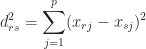
- Euclidian Distance:
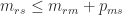
- Standardized Euclidian Distance:
- Mahalanobis Distance:
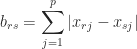
- Manhattan or City Block Metric:
- Minkowski Metric:
This distance is the most common in cluster analysis because it measures the geometric distance between two points in a n-dimensional space. It means that we can see if two points are near or far away in the geometric space. There is no difference if it is apply in a centered or non-centered variable. It is well used when the analyzed variables were measured under the same scale or there are no big differences between its scales. This distance is expressed as follow:
When the variables have different scales of measure, the euclidian distance is not a good dissimilarity index because it can be highly influenced by the variable with greatest scale. In this situation, the Standardized Euclidian Distance is a good alternative. As you see, this distance is similar to the euclidian distance but with weights to each variable.

It takes in consideration the difference in variance between features and their covariance structure. This distance is equivalent to applying the euclidian distance to the full principal components matrix.

You can note that this distance delete the covariance structure. That makes it non adequate in some occasions where the correlation is very important in the distance.
This distance is based in the sum of the absolute values of the differences among the coordinates. In this metric, a constant difference between each of the p coordinates in the amount 


The Minkowski metric is a more general distance that covers some of the distances presented above. When 

![\displaystyle m_{rs}=\left[\sum_{j=1}^p |x_{rj}-x_{sj}|^\lambda\right]^{1/\lambda}](https://s0.wp.com/latex.php?latex=%5Cdisplaystyle+m_%7Brs%7D%3D%5Cleft%5B%5Csum_%7Bj%3D1%7D%5Ep+%7Cx_%7Brj%7D-x_%7Bsj%7D%7C%5E%5Clambda%5Cright%5D%5E%7B1%2F%5Clambda%7D&bg=ffffff&fg=222222&s=0&c=20201002)
Similarity
Considering two objects 
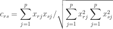
- Cosine:
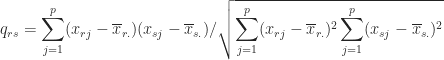
- Correlation coefficient:
In Multivariate Analysis, the cosine of the angle between two vectors is used as a kind of measurement of similarity. It only consider the direction of the two vectors and does not depend of the length of the vectors. This kind of measure is useful when you want to evaluate the structure of the profiles.
When the cosine is calculated to the centralized variable, it is known as the Pearson Correlation Coefficient.
For more information, you can check the book of J. D. Jobson, “Applied Multivariate Data Analysis: Volume II”. I hope this information will be useful for you.
Datos sin estadística
“Los datos, sin estadística, no son más que ruido y confusión.”
“Data, without statistics, it is not more than noise and confusion.”
¿Cómo actualizar Debian 7 Wheezy?
Debian 7 Wheezy es la última actualización estable de las distribución Debian en Linux. Hasta ahora me ha funcionado perfectamente y es por ello que deseo mostrar algunos pasos y sitios web que me funcionaron perfectamente para su actualización e instalaciones de programas que para mi caso son importantes.
0) Instalar de Debian 7 Wheezy:
Para los que desean instalar el Debian 7 Wheezy, descargar el instalador en http://www.debian.org/CD/http-ftp/, los tipos de descarga son CD y DVD. Los CDs son instaladores ligeros, requieren de conexión internet para su buena instalación mientras que los DVD son más completos y no requieren de conexión a internet para culminar la instalación.
1) Actualización de Debian Wheezy:
1.1) Preparamos nuestro sistema actual. Ejecutar los siguientes comando en la consola como superusuario:
aptitude update
aptitude upgrade
aptitude clean
Realizamos este paso porque se recomienda que no existan problemas de dependencias entre los paquetes. En caso contrario tratar de arreglar ello o intentar la actualización creando un backup como respaldo.
1.2) Actualizar la lista de repositorios para descargar e instalar los paquetes del Debian 7 Wheezy.
Para ello, se debe modificar el archivo /etc/apt/sources.list quedando de la siguiente manera.
deb http://ftp.us.debian.org/debian/ wheezy main
deb-src http://ftp.us.debian.org/debian/ wheezy main

deb http://security.debian.org/ wheezy/updates main contrib
deb-src http://security.debian.org/ wheezy/updates main contrib

# wheezy-updates, previously known as 'volatile'
deb http://ftp.us.debian.org/debian/ wheezy-updates main contrib
deb-src http://ftp.us.debian.org/debian/ wheezy-updates main contrib
1.3) Actualizar los paquetes de Debian 7 Wheezy.
apt-get update
apt-get upgrade
apt-get dist-upgrade
reboot
lsb_release -a
Como resultado debes obtener las características de tu nuevo debian instalado (Debian 7 Wheezy )
2) Links que funcionan para la instlación de los siguientes programas:
2.1) Software R: http://cran.r-project.org/bin/linux/debian/
Añadimos el siguiente repositorio a /etc/apt/sources.list.
# r backports
deb http://www.vps.fmvz.usp.br/CRAN/bin/linux/debian wheezy-cran3/
Ejecutamos los siguientes comando en el terminal como superusuario.
apt-key adv --keyserver subkeys.pgp.net --recv-key 381BA480
apt-get update
apt-get install r-base r-base-dev
2.2) IDE Rstudio: http://www.rstudio.com/ide/download/desktop
Instalar con GDebi Package Instaler haciendo anticlick en el paquete descargando y abriendo con GDebi.
2.3) Texstudio (Interface para el Editor de Textos Científicos Latex): http://packages.debian.org/wheezy/texstudio
Instalarlo por medio del Gestor de Paquetes. Sin embargo, la instalación no está completa, para el correcto funcionamiento añadir los paquetes recomendados y sugeridos en el link de esta sección.
2.4) Skype: http://wiki.debian.org/skype
Seguir los pasos del link, funciona y está completo.
2.5) Google Earth: http://diversidadyunpocodetodo.blogspot.com.es/2013/05/debian-wheezy-instalar-google-earth-64-ati-multiarch.html
Seguir los pasos del link pero no considerar el siguiente código porque el paquete ia32-libs ya no está disponible:
apt-get install ia32-libs
2.6) Mendeley Desktop (Gestor de bibliografías): http://www.mendeley.com/
Instalarlo por medio del Gestor de Paquetes.
2.7) Dropbox: https://www.dropbox.com/
2.8) Actualizar Iceweasel (Firefox): http://linuxgnublog.org/instalar-la-ultima-version-de-iceweasel-en-debian-wheezy/
Continuar con el link mostrado pero sólo agregar a /etc/apt/sources.list.
# mozilla backports
deb http://mozilla.debian.net/ wheezy-backports iceweasel-release
deb-src http://mozilla.debian.net/ wheezy-backports iceweasel-release
2.9) Actualizar Flash Player: http://permalink.gmane.org/gmane.linux.debian.user.spanish/180717
Agregar a /etc/apt/sources.list.
deb http://ftp.us.debian.org/debian wheezy contrib
Ejecutar en la consola, como superusuario:
apt-get update
apt-get install flashplugin-nonfree
Espero les sirva de ayuda, hasta la próxima.
Probabilidades de la vida
Este capítulo de Redes para la ciencia nos muestra que las probabilidades están en los sucesos que vivimos día a día. Aunque existen ciertos errores con las probabilidades y los porcentajes presentados, es una manera muy interesante y entretenida de hablar de probabilidades con todo el mundo…
Denle al enlace para que puedan ver este programa con Eduardo Punset y Amir Aczel…
http://www.redesparalaciencia.com/7252/redes/redes-125-descifrar-las-probabilidades-e-la-vida
¿Porqué usar la media armónica?
Recuerdo cuando llevé la clase de Estadística Descriptiva, y también la de Inferencia Paramétrica, nos presentaron estadísticos descriptivos como el promedio aritmético, geométrico y armónico. En ese instante no tenía ni la mas vaga idea de cuando utilizar el promedio armónico ya que al parecer, no podía interpretar, aquella fórmula, de una manera más comprensible o que de pistas de una interpretación clara tal como lo es el promedio aritmético. Cuento esto, porque me imagino que muchos se sienten identificados y por ello quiero compartir un ejemplo que hace un tiempo atrás revisé, espero que resulte de su interés. Es el siguiente:
Imagine que se esta estudiando la velocidad promedio de los vehículos en una vía definida, de la cual se tiene conocimiento de su longitud o distancia 


En donde 


Además recuerde que:

En donde 

Ahora reemplazando (2) en (1).

La constante d se elimina y obtenemos:

lo cual viene a ser el promedio armónico. Conocido como velocidad-promedio espacio en la Simulación de Tráfico.
